Chicago Crime Investigation Final Report

Team KungFu Pandas: Raj Patel, Ayush Jamindar, Amrita Rajesh, Saloni Mhatre, Lakshmi Krishna

link to the notebook - https://github.com/uic-cs418/group-project-kungfu-pandas/blob/main/Final_Report.ipynb

Project Introduction

We are analyzing two datasets involving Chicago crime and housing. The crime dataset and housing dataset are publicly available at :

• Chicago Crime Data Source: https://data.cityofchicago.org/Public-Safety/Crimes-2001-to-Present/ijzp-q8t2/about_data
• Zillow Data Source: https://www.zillow.com/research/data/

Our inquiries: Which neighborhood is the least safe to move into? Is there a relationship between housing prices and crime in Chicago? Has crime rates increased after post-covid compare to pre-covid? What are the most common type of crime committed in Chicago area?

Initial hypotheses: There is a negative correlation between crime activity and house prices. As time progresses, crime will increase.

IMPORTANT NOTE:

Please create a folder called `csv_files`. This will contain all the CSV files so after downloading the data, please put it in this folder.

import pandas as pd
import numpy as np
from CleaningPR import *
from ML_pr import *
from Visualization1 import *
from Visualization2_Battery import *
from Visualization2_Theft import *
from Visualization3_Battery import *
from Visualization3_Theft import *
from t_test import *
from EDA_pr import *
from sklearn.linear_model import LogisticRegression
from sklearn.preprocessing import OneHotEncoder

Data Cleaning Process

The following steps are to manipulate and clean the datasets. After obtaining the size, dimensions, and summary of the data, some columns and rows were dropped, more features were added, and dataframes were combined to be stored into seperate CSV files for easy access.

• The crime dataset contains information about the reported crimes that took place in Chicago from January 2001 to February 2024
• Granularity: Each row in this data represents individual crimes with details about each crime such as ID, Case Number, Date etc.
• Data contains ~8 million records and will go to ~1.4 million records after filtering
• First, the dates were converted to a timestamp, then the unecessary columns were dropped such as block, latitide, longitude etc. Next, the data was filtered and then the resulting dataframe was saved into the following seperate CSV files: (Crimes_2017_to_2019.csv, Crimes_2021_to_Present.csv, Crimes_2014.csv)

crime_data = pd.read_csv('csv_files/Crimes_2001_to_Present.csv')

'''
    cleanCrimeData method will perform Step 1,2,3 and 4.
    if want to see the cleaned version of pre-covid, post-covid crime data and decade crime data
    then try opening and printing the head of `Crimes_2017_to_2019.csv`, `Crimes_2021_to_Present.csv`, `Crimes_2014.csv`
'''
cleanCrimeData(crime_data)

Columns:  ['ID', 'New_Date', 'Primary Type', 'Location Description', 'Arrest', 'Community Area', 'RegionName']

Neighborhood Dataset Information and Cleaning

• The data below is from Zillow and it shows the average house price for each nighborhood in the country
• Granularity: Each row represents a neighborhood in a state and shows the average house price for each month from 1-31-2000 to 1-31-2024
• Contains average monthly prices for real estate of around ~21000 neighborhoods across the U.S. and filters down to 181 neighborhoods in Chicago
• First, the data from Chicago neighborhoods specifically was extracted. Next, the data was transposed by reseting the index, rotating the dataframe to flip the columns and rows and allows for easier manipulation. Finally the dataframe was filtered for pre and post covid and saved into (neighborhood_data_2017_to_2019.csv, neighborhood_data_2021_present.csv)

neighborhood_data = pd.read_csv('csv_files/Neighborhood_House_Price.csv')

''' cleanHousingData method will perform Step 1,2,and 3. 
    if want to see the cleaned version of pre-covid and post-covid data then 
    try opening and printing the head of `neighborhood_data_2017_to_2019.csv`, `neighborhood_data_2021_present.csv` '''
cleanHousingData(neighborhood_data) 

Exploratory Data Analysis

Neighborhood Data Exploration

Exploring the neighborhood dataset, we seperated the dataset into two CSV files for pre and post Covid.
Between 2017 and 2019, neighborhood prices were like this: the average minimum was about \$ 227,167, and the average maximum was roughly \$ 255,476. Median for the minimum price was \$ 212,369 and for maximum price was \$ 242,843. The cheapest house was in Golden Gate, selling for \$ 25,263 in January 2017, while the most expensive was in North Center, priced at \$ 585,357 in May 2018. In terms of neighborhoods, Golden Gate was the cheapest, averaging about \$ 37,259, while North Center was the most expensive, averaging around \$ 573,486. The month with the most crime commited is July with 73,950 incidents and the month with the least is February with 54,432 incidents.

Since 2021, neighborhood prices have risen slightly, with average minimums around \$ 264,326 and maximums hitting about \$ 299,737. The cheapest house, in Golden Gate, was priced at \$ 55,618 in January 2021, while the most expensive, in North Center, was priced at \$ 696,986 in November 2023. Ford City is the most affordable neighborhood, averaging around \$ 68,129, whereas Ravenswood Manor is the most expensive, averaging approximately \$ 655,319. The month with the most crime commited is January with 70,657 incidents and the month with the least is February with 51,792 incidents.

neighborhood_2017_2019 = pd.read_csv('csv_files/neighborhood_data_2017_2019.csv')
neighborhood_2021_present = pd.read_csv('csv_files/neighborhood_data_2021_present.csv')
crime_data1 = pd.read_csv('csv_files/Crimes_2017_to_2019.csv')
crime_data2= pd.read_csv('csv_files/Crimes_2021_to_Present.csv')

# To see the output you can uncomment one by one to see
# get_neighborhood_price_stats(neighborhood_2017_2019)
# get_neighborhood_price_stats(neighborhood_2021_present)

Crime Data Exploration

For the years 2017-2019, the least common crime type is arson, while the most common is weapons violation. Edison Park had the fewest arrests, totaling 79, whereas Austin had the most, with a staggering 11,443 arrests. For overall crime, Edison Park had the lowest number, with 777 incidents, while Austin had the highest, with 44,856 incidents. The top five locations for crime include streets with 174,926 incidents, residences with 131,615 incidents, apartments with 101,710 incidents, sidewalks with 62,242 incidents, and other locations with 31,925 incidents. On the other hand, the top five locations with the least crime each had only one incident: YMCA, railroad property, rooming house, office, and nursing home.

From 2021 onwards, The least common crime is arson, while the most common is weapons violation. Edison Park had the fewest arrests, totaling 63, while Austin had the most, with 5,743 arrests. For overall crime, Edison Park had the lowest number, with 838 incidents, while Austin had the highest, with 37,281 incidents. The top five locations for crime include streets with 203,027 incidents, apartments with 141,976 incidents, residences with 95,109 incidents, sidewalks with 37,672 incidents, and parking lots/garages (non-residential) with 26,416 incidents. On the other hand, the top five locations with the least crime each had only one incident: farm, banquet hall, CTA subway station, elevator, and basement.

# These are the EDA functions which contain the code, feel free to uncomment and run them :)
# get_crime_stats(crime_data1)
# get_crime_stats(crime_data2)

Machine Learning

We began by splitting the decade crime data from crime_data_2014.csv into training and testing sets to ensure we didn't touch the testing data initially. Next, we determined the best feature(s) for predicting arrest probability using logistic regression. This involved encoding string variables into 0s and 1s for easier model fitting, employing k-fold cross-validation to evaluate model performance, and ultimately selecting the feature combination yielding the highest accuracy.

Comparing our logistic regression model, which incorporates Primary Type, Location Description, and RegionName, against a baseline model using mode prediction, we found an 87% accuracy improvement with the logistic regression model.

Then, we trained the LogisticRegression Model using the best feature determined earlier on the same training set, avoiding the creation of a new one. This involved training the model, testing it, and creating a new dataframe for further analysis.

crime_data_2014 = pd.read_csv('csv_files/Crimes_2014.csv')
'''
    Step 1: Spliting
'''
X = crime_data_2014[['Primary Type', 'Location Description', 'RegionName']]
y = crime_data_2014['Arrest'] 
X_train, X_test, y_train, y_test = train_test_split(X, y, test_size=0.2, random_state=42) # 80% training, 20% testing
print("length of the training dataset",len(X_train))

'''
    best_feature method will perform step 2 and 3
'''
feature = best_feature(crime_data_2014, X_train, y_train)

''' train_test method will perform step 4 '''
train_test(X_train, X_test, y_train, y_test, feature) # Uses Logistic Regression Model to train and test our model

length of the training dataset 2008524
Best Features ['Primary Type', 'Location Description', 'RegionName'] Accuracy of Logistic Regression:  0.8786626398290486
Accuracy of the baseline model:  0.8083941242424786
Accuracy of the model on the test dataset: 0.8786813029243307

	Primary Type	Location Description	RegionName	Prob
2178855	THEFT	SIDEWALK	Loop	0.071568
1869478	ASSAULT	ALLEY	Lake View	0.112260
1299827	THEFT	SIDEWALK	Englewood	0.076976
1024670	THEFT	SIDEWALK	West Town	0.054855
229033	BATTERY	STREET	Near South Side	0.200898

Model Usage

Firstly we trained our model using the crime data from the past decade(2014-present) so that it can learn as much as possible. Then our stakeholder Residents of Chicago, UIC students, new settlers and Chicago Police Department can predict the probabilty of a person getting arrested based on the type of crime, neighborhood, and description of the location. This will be beneficial to determine how safe a neighborhood is. Our model will not give 100% accuracy on the prediction but it will predict the outcome 87.86% of the time correctly, this is significant becuase our model is not overfitting. In other terms, it be able to predict almost 9 out of 10 outcomes correctly.

Visualizations

Theft and Battery are the most frequently committed crimes

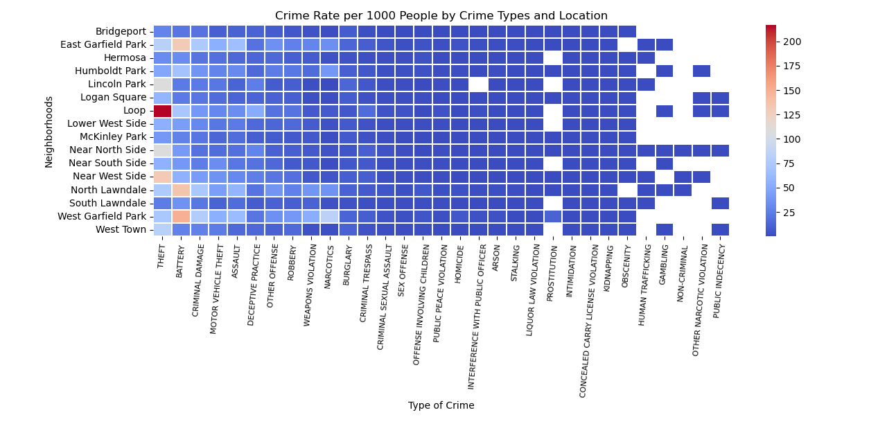
Findings: Heatmap

This heatmap looks at frequency of crime in the top 16 closest neighborhoods to UIC. The populations of neighborhoods are standardized by calculating the crime rate per 1000 people and the types of crimes were arranged from most to least frequent. This visualization shows that theft and battery are the most frequently committed crimes especially in the Loop for the former and North Lawndale and West Garfield Park for the latter. This information led to inquiries about whether the affluence of a neighborhood had an effect on theft and battery.

In theft, there is no apparent relationship between crime quartiles and housing price

In battery, as crime quartile increases, housing price goes down

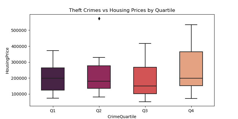
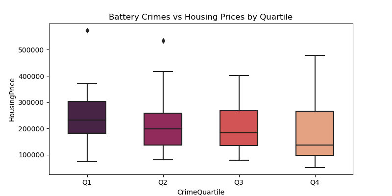
Findings: Boxplots

These boxplots show housing price on the y-axis and crime was divided into four quartiles on the x-axis. Theft and battery were the main focuses as they were the most frequently committed crimes. For theft, there is no apparent relationship between theft and housing prices. However for battery, it seems that as the housing prices go up, there is less battery. This leads to the conclusion that the most battery occurs in the less wealthy neighborhoods.

There is a significant decrease in theft between post-covid compared to pre covid

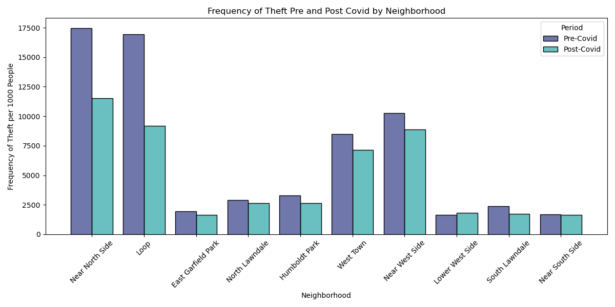
This histogram looks at frequency of theft from pre to post covid. The populations of neighborhoods are again standardized by calculating the crime rate per 1000 people and the the x axis shows the changes in the top 10 closest neighborhoods to UIC. There seems to be a sizable decrease in theft post covid compared to precovid, so a t-test was performed to test if that was the case (shown below). The p value < 0.05 and the tstat > 0 so the null hypothesis was rejected and a conclusion was drawn our initial hypothesis was wrong: there is a significant decrease in theft post COVID compared to pre COVID.

Statistical Analysis

pre = pd.read_csv('csv_files/Crimes_2017_to_2019.csv')
post = pd.read_csv('csv_files/Crimes_2021_to_Present.csv')
ttest_uic_theft(pre, post)

3.294241116171095 0.009315091584718934
Reject the NULL Hypothesis: There is a significant decrease in theft post COVID compared to pre COVID

There is no significant change in battery between post-covid compared to pre covid

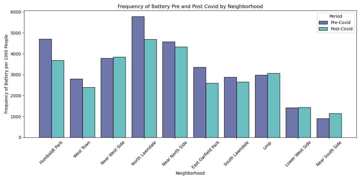
This histogram looks at frequency of battery from pre to post covid. The populations of neighborhoods are again standardized by calculating the crime rate per 1000 people and the the x axis shows the changes in the top 10 closest neighborhoods to UIC. There does not seem to be a significant change between precovid and postcovid and a t-test was performed to confirm that (shown below). The p value was greater 0.05 so there was not sufficient enough proof to reject the null hypothesis and a conclusion was drawn our initial hypothesis was wrong: there is no significant change in battery between pre and post covid.

ttest_uic_battery(pre, post)

1.5145965886948978 0.16417466325645683
Fail to reject the NULL hypothesis: There is no significant difference in battery between pre and post covid

Main Takeaways

• Theft and battery were the most frequently committed crimes out of all the crimes done in Chicago
• There is inverse relationship between housing prices and battery (Expensive houses tends to have lower battery cases)
• There is no direct relationship between housing prices and theft (Expensive houses still tend to have higher theft crime compare to cheaper houses)
• There has been a decrease in theft post covid compared to pre covid in the neighborhoods near UIC
• There was no significant change in battery between pre and post covid near UIC
• Our model is able to predict about 88% accurately about the outcome of arrest based on type of crime, neighborhood and description of crime.

END OF REPORT